Part 1: The Roots – Recurrent Neural Networks (RNNs)
Series: From Sequences to Sentience: Building Blocks of the Transformer Revolution
Subtitle: Why the First Neural Networks for Sequences Had Promise—and Limitations
Introduction: The Dawn of Sequence Modeling
Imagine teaching a computer to predict the next word in a sentence, translate a foreign language, or compose music note by note. These tasks all involve sequences—data where order matters. In the early days of deep learning, Recurrent Neural Networks (RNNs) were the go-to solution for handling such sequential data. Introduced in the 1980s and refined over decades, RNNs laid the groundwork for modern AI language models by giving machines a rudimentary sense of "memory." But as we’ll see, their promise came with serious limitations that paved the way for more advanced architectures.
This article, the first in an 8-part series, explores how RNNs work, why they were revolutionary, and why they ultimately fell short of the demands of modern AI.
What is a Recurrent Neural Network?
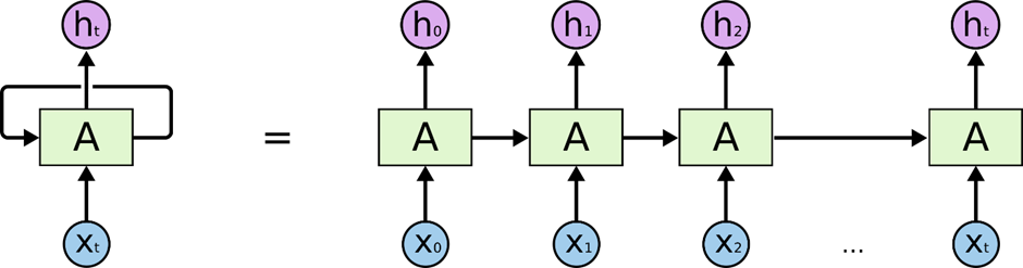
Unlike standard neural networks, which process inputs independently, RNNs are designed for sequential data like text, speech, or time series. Their key feature is a feedback loop: at each step, the RNN combines the current input with a hidden state—a summary of everything it has seen so far—to produce an output and update its memory.
This makes RNNs well-suited for tasks such as:
- Predicting the next word in a sentence (e.g., auto-complete in texting).
- Translating languages (e.g., "Hello" to "Bonjour").
- Generating sequences like music or code.
- Forecasting time series data (e.g., stock prices).
Unlike standard neural networks, which process inputs independently, RNNs are designed for sequential data like text, speech, or time series. Their key feature is a feedback loop: at each step, the RNN combines the current input with a hidden state—a summary of everything it has seen so far—to produce an output and update its memory.

Key Idea: Memory Through Recurrence
The hidden state acts like a short-term memory, carrying information from one step to the next. Mathematically, for a given time step ( t ), the RNN computes the new hidden state ( h_t ) as:
[ h_t = \tanh(W_{xh}x_t + W_{hh}h_{t-1} + b) ]
- ( x_t ): Current input (e.g., the word "love").
- ( h_{t-1} ): Previous hidden state (memory of prior words).
- ( W_{xh}, W_{hh} ): Weight matrices for input and hidden state.
- ( b ): Bias term.
- ( \tanh ): Activation function to keep values manageable.
This recurrence allows RNNs to theoretically "remember" earlier parts of a sequence and use them to inform future predictions.
Example: Predicting Text with an RNN
To make this concrete, consider teaching an RNN to predict the next word in the sentence: "I love deep learning."
- Step 1: The RNN sees "I" and initializes its hidden state.
- Step 2: It processes "love," combining it with the memory of "I" to update the hidden state and predict the next word.
- Step 3: It sees "deep," using the memory of "I love," and so on.
Over time, the RNN learns temporal dependencies—for example, that "love" is more likely to follow "I" than "banana." This ability to model sequence patterns made RNNs exciting for early NLP applications.
Below is a simplified Python example using PyTorch to show how an RNN might process this sentence:
import torch
import torch.nn as nn

# Simple RNN model
class SimpleRNN(nn.Module):
    def __init__(self, input_size, hidden_size, output_size):
        super(SimpleRNN, self).__init__()
        self.rnn = nn.RNN(input_size, hidden_size, batch_first=True)
        self.fc = nn.Linear(hidden_size, output_size)

    def forward(self, x, hidden):
        out, hidden = self.rnn(x, hidden)
        out = self.fc(out)
        return out, hidden

# Example parameters
vocab = {"I": 0, "love": 1, "deep": 2, "learning": 3}
input_size = len(vocab)  # Vocabulary size
hidden_size = 10         # Size of hidden state
output_size = len(vocab) # Output is next word prediction

# Initialize model
model = SimpleRNN(input_size, hidden_size, output_size)

# Input: "I love deep" as one-hot vectors
sequence = ["I", "love", "deep"]
input_tensor = torch.zeros(1, len(sequence), input_size)
for i, word in enumerate(sequence):
    input_tensor[0, i, vocab[word]] = 1

# Initial hidden state
hidden = torch.zeros(1, 1, hidden_size)

# Forward pass
output, hidden = model(input_tensor, hidden)
print("Output shape:", output.shape)  # Predicts next word probabilities
# Forward pass
output, hidden = model(input_tensor, hidden)
print("Output shape:", output.shape)  # Predicts next word probabilities
This code demonstrates a basic RNN predicting the next word in a sequence, capturing the essence of recurrence.
The Limitations of RNNs
Despite their theoretical strengths, RNNs faced significant challenges that limited their practical use:
- Vanishing and Exploding Gradients
During training, RNNs rely on gradients to update weights. Because the same weights are reused across time steps, gradients can either vanish (become too small) or explode (become too large). This makes it hard for RNNs to learn long-term dependencies. For example, in the sentence:
"The cat, which was black and fierce and came out only at night, slept,"
the RNN struggles to connect "slept" back to "cat" due to the long gap. - Sequential Processing
RNNs process one token at a time, like reading a book word by word. This sequential nature prevents parallelization, making training slow, especially on GPUs designed for parallel tasks. Long sequences or large datasets exacerbate this issue. - Short-Term Memory Bias
Even when trained successfully, RNNs tend to focus on recent tokens, forgetting earlier ones. This bias limits their ability to maintain context over long sequences.
Table: Strengths and Weaknesses of RNNs
| Aspect | Strength | Weakness |
| Sequence Handling | Captures temporal dependencies | Struggles with long-term dependencies |
| Training Speed | Simple for short sequences | Slow due to sequential processing |
| Scalability | Works for small datasets | Poor scaling for long sequences or corpora |
| Memory | Theoretical long-term memory | Biases toward recent tokens |
Attempts to Improve RNNs
Researchers developed several variants to address RNN limitations:
- Bidirectional RNNs: Process sequences forward and backward, improving context for tasks like speech recognition.
- Stacked RNNs: Use multiple RNN layers to capture richer patterns, increasing model capacity.
- Gated RNNs (GRUs, LSTMs): Introduce gates to control what to remember or retain, helping with long-term dependencies (covered in Part 2).
These variants were improvements, but they remained workarounds rather than fundamental solutions. RNNs were still too slow and limited for the ambitious language models researchers dreamed of.
RNNs: A Foundation for the Future
RNNs were a critical stepping stone in the evolution of AI. They introduced the idea of modeling sequences with memory, powering early applications like Google Translate, speech recognition, and simple chatbots. But their flaws—slow training, short memory, and unstable learning—made it clear they couldn’t scale to handle the complex, fluent, context-aware language processing we expect from modern AI.
The stage was set for a new approach, one that could process sequences faster, capture global context, and scale to massive datasets. That breakthrough would arrive with the Transformer architecture, but first, we’ll explore the refinements of RNNs in Part 2.
Featured Blogs
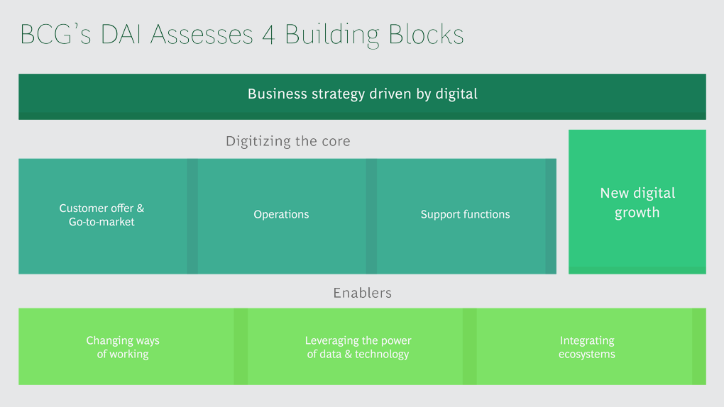
BCG Digital Acceleration Index

Bain’s Elements of Value Framework
McKinsey Growth Pyramid
McKinsey Digital Flywheel
McKinsey 9-Box Talent Matrix
McKinsey 7S Framework
The Psychology of Persuasion in Marketing

The Influence of Colors on Branding and Marketing Psychology

What is Marketing?
Recent Blogs
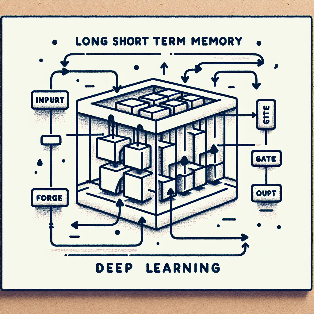
Part 2: The Gatekeeper – Long Short-Term Memory (LSTM) Networks

Part 1: The Roots – Recurrent Neural Networks (RNNs)
How Hierarchical Priors Helped Anita Make Smarter, Faster Marketing Decisions
Demystifying SHAP: Making Machine Learning Models Explainable and Trustworthy
Survival Analysis & Hazard Functions: Concepts & Python Implementation