Part 2: The Gatekeeper – Long Short-Term Memory (LSTM) Networks
Series: From Sequences to Sentence: Building Blocks of the Transformer Revolution
Can We Give RNNs a Better Memory?
Introduction: A Smarter Memory for Sequences
In Part 1, we explored how Recurrent Neural Networks (RNNs) introduced the idea of memory for processing sequences like text or time series. However, their tendency to forget long-term information due to vanishing gradients limited their potential. Enter Long Short-Term Memory (LSTM) networks, introduced by Hochreiter and Schmidhuber in 1997. LSTMs were a breakthrough, equipping RNNs with a sophisticated memory system to retain context over longer periods. This article, the second in an 8-part series, dives into how LSTMs work, their strengths, and why they were a stepping stone rather than the final destination.
The LSTM Innovation: Memory That Lasts
Imagine an RNN as a person with a short attention span, forgetting details from the start of a long story. LSTMs address this "forgetfulness" by introducing a cell state—a conveyor belt of information that runs through the network—paired with gates that control what to keep or discard. This design tackles the vanishing gradient problem, allowing LSTMs to remember details over dozens or even hundreds of steps, far surpassing standard RNNs.
Think of an LSTM as an RNN with a smart memory controller, deciding what to hold onto and what to let go.
Key Components of an LSTM Cell
An LSTM cell is a complex unit with four interacting layers, each governed by a gate. These gates use sigmoid functions (outputting values between 0 and 1) to regulate the flow of information. Here’s how they work:
- Forget Gate
Decides what to discard from the cell state.
![]()
 : Previous hidden state
- xt: Current input
- Wf, bf: Weight matrix and bias
- Output ft (0 = forget, 1 = keep).
- Input Gate
Determines what new information to store in the cell state. It has two parts:

![]()
- it: Controls which values to update.
 : Candidate values to add to the cell state.
- Cell State Update
Combines the forget and input gates to update the cell state:
 : Previous cell state.
This step either keeps old information or adds new insights.
- Output Gate
Decides what to output based on the cell state:

![]()
- ot: Filters the cell state for output.
- ht: New hidden state sent to the next step.
Together, these components allow the LSTM to learn what to remember, what to forget, and what to share.

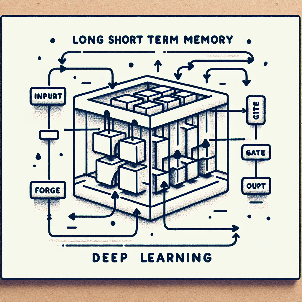
Fig: LSTM Cell Diagram: The cell state and gates manage memory across time steps.


How It Works – Intuition
Picture the cell state as a conveyor belt moving through time, carrying essential information like a story’s main character. The gates act as valves:
- The forget gate removes irrelevant details (e.g., minor side notes).
- The input gate adds new, relevant information (e.g., the character’s actions).
- The output gate decides what to reveal at each step (e.g., the current plot point).
Unlike RNNs, which overwrite their hidden state at every step, LSTMs preserve and refine their cell state, making them far better at maintaining context.
Example: Long-Term Memory in Action
Consider the sentence: "The cat, which had walked through the garden, finally curled up."
An LSTM can remember "cat" 12 tokens later when processing "curled up," while an RNN would likely lose track due to the long gap.
Real-World Use Cases
Before the transformer era (pre-2018), LSTMs were the gold standard for sequence modeling:
- Google Translate (early versions): Powered initial language translation.
- Speech Recognition: Used in Apple Siri and Amazon Alexa.
- Time-Series Forecasting: Applied in finance and energy sectors.
- Music Generation: Created melodies by learning patterns.
Strengths and Limitations
Strengths
- Handles Long-Term Dependencies: Excels at remembering context over many steps.
- Better Gradient Flow: The cell state stabilizes training by avoiding vanishing gradients.
- Excellent for Medium-Length Sequences: Ideal for tasks like sentence-level translation.
- Interpretability: Gates provide insight into what the model learns.
Limitations
- Still Sequential: Processes data one step at a time, preventing parallelization.
- Computationally Expensive: Multiple gates per step increase processing demands.
- Training Challenges: Can still struggle with very long texts.
- Limited Scalability: Doesn’t handle massive datasets or billions of tokens efficiently.
Table: LSTM Strengths and Limitations
| Aspect | Strength | Limitation |
| Memory | Retains long-term dependencies | Struggles with very long texts |
| Training Stability | Improves gradient flow | Training can be complex |
| Speed | Good for medium sequences | Sequential, no parallelism |
| Scalability | Works for moderate data | Poor for massive datasets |
LSTM in Code
Here’s a practical example using PyTorch to demonstrate an LSTM processing a sequence:
import torch
import torch.nn as nn

# Define a simple LSTM model
input_size = 10    # Example input feature size
hidden_size = 20   # Hidden state size
num_layers = 2     # Number of LSTM layers
lstm = nn.LSTM(input_size, hidden_size, num_layers, batch_first=True)

# Sample input: (batch_size, sequence_length, input_size)
input_sequence = torch.randn(1, 5, input_size)  # 1 batch, 5 time steps
hidden = torch.zeros(num_layers, 1, hidden_size) # Initial hidden state
cell = torch.zeros(num_layers, 1, hidden_size)   # Initial cell state

# Forward pass
output, (hn, cn) = lstm(input_sequence, (hidden, cell))

# Output shapes
print("Output shape:", output.shape)  # [1, 5, 20] - predictions for each step
print("Hidden state shape:", hn.shape)  # [2, 1, 20] - final hidden state
print("Cell state shape:", cn.shape)    # [2, 1, 20] - final cell state
Sample Output
Running this code produces:
Output shape: torch.Size([1, 5, 20])
Hidden state shape: torch.Size([2, 1, 20])
Cell state shape: torch.Size([2, 1, 20])
- Output: Contains predictions for each of the 5 time steps, with 20 features per step (hidden size).
- Hidden State (hn): The final hidden state from all layers.
- Cell State (cn): The final cell state, reflecting the LSTM’s memory.
- Note: This is an untrained model, so values are random. Training on data would refine these outputs.
LSTM Set the Stage – But Not the Future
LSTMs demonstrated that enhancing memory could unlock better sequence understanding, powering many early AI successes. However, the growing demand for:
- Faster training through parallel processing,
- Longer context windows for richer context,
- Scalability to handle billions of tokens,
outstripped LSTM’s capabilities. Its sequential nature and computational cost made it a clever fix for RNNs, not a platform for the massive scale of modern language models.
The search for a new architecture continued, leading us to the next milestone.
Up Next: Part 3 – Word Embeddings: Giving Words Meaning
Before transformers could shine, we needed a way to represent words as meaningful numbers. In the next part, we’ll explore Word2Vec, GloVe, and the rise of semantic embeddings that laid the foundation for advanced language models.
Featured Blogs
BCG Digital Acceleration Index

Bain’s Elements of Value Framework
McKinsey Growth Pyramid
McKinsey Digital Flywheel
McKinsey 9-Box Talent Matrix
McKinsey 7S Framework

The Psychology of Persuasion in Marketing

The Influence of Colors on Branding and Marketing Psychology

What is Marketing?
Recent Blogs
Part 2: The Gatekeeper – Long Short-Term Memory (LSTM) Networks

Part 1: The Roots – Recurrent Neural Networks (RNNs)
How Hierarchical Priors Helped Anita Make Smarter, Faster Marketing Decisions

Demystifying SHAP: Making Machine Learning Models Explainable and Trustworthy
Survival Analysis & Hazard Functions: Concepts & Python Implementation